This week's topics covered the chi-square test and corresponding visualization.
Question # 1 : The following table is the contingency table that displays the actual data from the hotel guest satisfaction study. The hotel is located on St. Pete beach. Using R, conduct Chi Square test and summaries the result using any type of visualization (basic, Lattice or ggplot2) to indicate if df is bigger 4 or smaller.
Null hypothesisH0: The degrees of freedom for the chi-square test is at least 4.
Alternative hypothesis
H1: The degrees of freedom for the chi-square test is less than 4.
#Input provided data
> data <- read.csv("hoteldata.csv", header=T)
#Run chi-square test on subdata frame
> chisq.test(data[1:2,2:3])
Pearson's Chi-squared test with Yates'
continuity correction
data: data[1:2, 2:3]
X-squared = 8.4903, df = 1, p-value = 0.00357
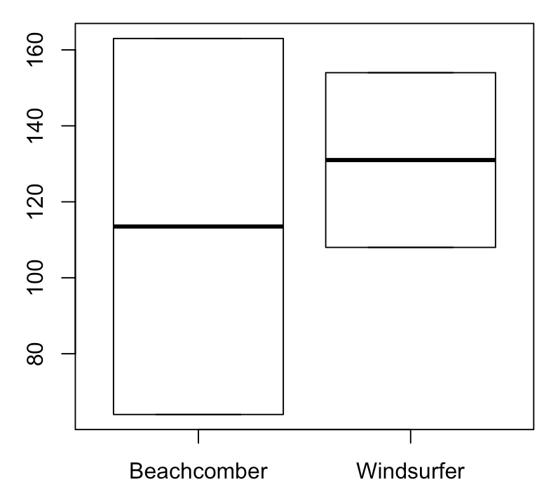
#Visualize data
> install.packages("lattice")
> library(lattice)
> boxplot(data[1:2,2:3])
Based on the results from the chi-square test, the degrees of freedom was 1. Therefore, we reject the null hypothesis.
Answer sheet :
> beach <- c(163, 64, 227)
> wind <- c(154, 108, 262)
> choice <- c("Yes", "No", "Total")
> d <- data.frame(choice, beach, wind)
> d$Total <- d$beach + d$wind
> d <- d[,-1]
> rownames(d) <- c("Yes", "No", "Total")
> d
beach wind Total
Yes 163 154 317
No 64 108 172
Total 227 262 489
> res <- chisq.test(d[1:2, 1:2])
> res
Pearson's Chi-squared test with Yates'
continuity correction
data: d[1:2, 1:2]
X-squared = 8.4903, df = 1, p-value = 0.00357
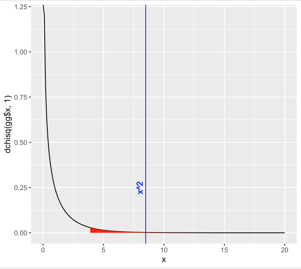
> gg <- data.frame(x = seq(0, 20, 0.1))
> View(gg)
> gg$y <- dchisq(gg$x, 1)
> ggplot(gg) + geom_path(aes(x,y)) +
geom_ribbon(data =
gg[gg$x>qchisq(0.05,1,lower.tail=FALSE),],
aes(x,ymin=0,ymax=y), fill="red") +
geom_vline(xintercept =
res$statistic, color="blue") +
labs(x = "x", y = "dchisq(gg$x, 1)") +
geom_text(aes(x=8, label="x^2", y=0.25),
color = "blue", angle=90)