This week I reviewed descriptive statistics and summarizing datasets via measurements of central tendency. This included the mean, median, mode, quartile ranges, variance, and standard deviation.

These topics in central tendency and distribution were mostly review, however, their application in R was interesting to learn and apply in R Studio. The language itself has considerable differences, in terms of syntax, from the previous languages I have practiced with (HTML, CSS, PHP, SQL). Despite these differences, R seems to be logical in its structure and hasn't presented me with any abnormal difficulties.

The below code from R Studio represents my assignment to find the "mean, median, and more" of 2 sets of integers:

  > x <- c(10, 2, 3, 2, 4, 2, 5) #define set 1
  > y <-c(20, 12, 13, 12, 14, 12, 15) #define set
  > mean(x); mean(y)
    [1] 4
    [1] 14
  > median(x); median(y)
    [1] 3
    [1] 13
  > sum(x); sum(y)
    [1] 28
    [1] 98
          

The below code from R Studio represents my assignment to find the "range, interquartile, variance, and standard deviation" of the same sets:

  > range(x); range(y)
    [1]  2 10
    [1] 12 20
  > IQR(x); IQR(y)
    [1] 2.5
    [1] 2.5
  > var(x); var(y)
    [1] 8.333333
    [1] 8.333333
  > sd(x); sd(y)
    [1] 2.886751
    [1] 2.886751
          

The mean of both sets distinguishes the average magnitude for each, indicating that Set 1 is composed of generally smaller numbers. This is further supported by the median and sum of the sets. However, the distribution between the sets is identical in terms of variance and standard deviation. The average scatter of the sets match despite their difference in value magnitudes.

The module video presentation covered descriptive statistics, specifically, the functions displayed above.

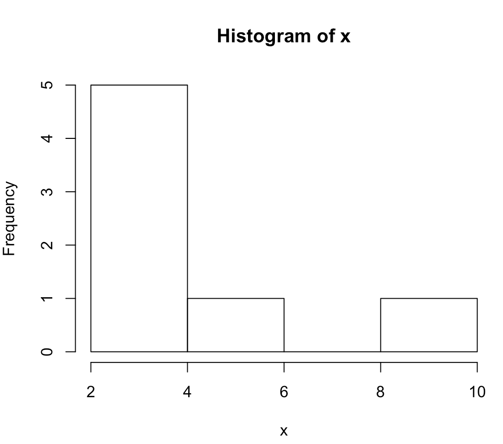
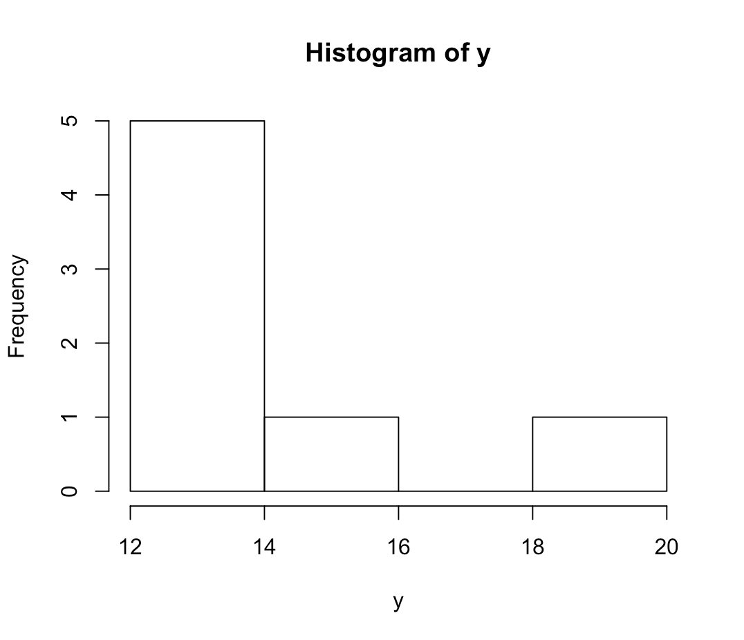
The diagrams below show graphics of histograms from the sets, using the R histogram function:

  > hist(x)
  > hist(y)
          

---