This week's topic included bivariate analysis, the analysis of two variables (often denoted as X and Y) for the purpose of determining
the type of relationship between them. Specifically, we utilized R to illustrate a Pearson's sample correlation and a Spearman's rank correlation.
The following data represent airport pre-boarding screener's during 1988 - 1999.
This data set includes two variables:
- # of pre-boarding screener's conducted, and
- # of security violations found in those scenarios
The following are measurements for the 20 random cases:
| Case | Pre-Boarding Screeners |
Security Violations Detected |
|---|---|---|
| 1 | 287 | 271 |
| 2 | 243 | 261 |
| 3 | 237 | 230 |
| 4 | 227 | 225 |
| 5 | 247 | 236 |
| 6 | 264 | 252 |
| 7 | 247 | 243 |
| 8 | 247 | 247 |
| 9 | 251 | 238 |
| 10 | 254 | 274 |
| 11 | 277 | 256 |
| 12 | 303 | 305 |
| 13 | 285 | 273 |
| 14 | 254 | 234 |
| 15 | 280 | 261 |
| 16 | 264 | 265 |
| 17 | 261 | 241 |
| 18 | 292 | 292 |
| 19 | 248 | 228 |
| 20 | 253 | 252 |
| N = 20 measurements | Mean boarding screeners = 261.2 | Mean security violations = 252.5 |
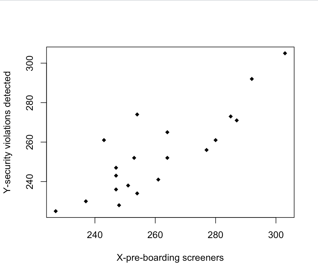
Question # 1 Describe the association between boarding screeners and security violations.
The number of boarding screeners (X) and number of security violations (Y) are discrete values, similar in magnitude for each entry. The number of security violations occasionally equals the number of screeners, but never exceeds it.
The correlation analyses below shed more light on their relationship. The resulting scatterplot indicates a positive correlation where increasing values of X result in increasing values of Y.
Question # 2 : Calculate Pearson’s Sample correlation coefficient using R.
  > screenings <- read.table(file.choose(),header=T,sep="\t")
  > head(screenings)
    pre.boarding.screeners security.violations.detected
  1                    287                          271
  2                    243                          261
  3                    237                          230
  4                    227                          225
  5                    247                          236
  6                    264                          252
  > cor.test(screenings[,1],screenings[,2])

  	Pearson's product-moment correlation

  data:  screenings[, 1] and screenings[, 2]
  t = 6.5033, df = 18, p-value = 4.088e-06
  alternative hypothesis: true correlation is not equal to 0
  95 percent confidence interval:
   0.6276251 0.9339189
  sample estimates:
        cor
  0.8375321
Question # 3: Calculate Spearman’s Rank Coefficient using R.
  > cor.test(screenings[,1],screenings[,2], method="spearman")

  	Spearman's rank correlation rho

  data:  screenings[, 1] and screenings[, 2]
  S = 322.47, p-value = 0.0001096
  alternative hypothesis: true rho is not equal to 0
  sample estimates:
        rho
  0.7575423

  Warning message:
  In cor.test.default(screenings[, 1], screenings[, 2],
method = "spearman") :
    Cannot compute exact p-value with ties
Question # 4 Create Scatter plot using R. The code for Scatter plot in R:
  > plot(screenings[,1],screenings[,2],pch=18,
          xlab="X-pre-boarding screeners",
          ylab="Y-security violations detected")